Project Instructions

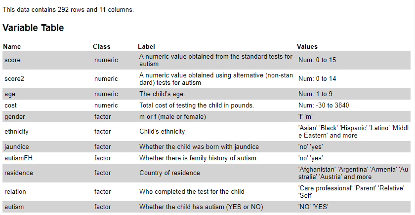
You will work with the child.csv file, which is a modified dataset adapted from the autism dataset available on Kaggle. This dataset contains attributes/variables for several children who were tested for autism.

Your task is to perform the following data analysis activities using R and Python.

Autism Data

To follow along with this tutorial, you can download the dataset in either Excel or CSV format by clicking the respective button.

Figure 1 shows the data dictionary for the child autism dataset.

A table presenting the data dictionary for a child autism dataset. The table includes columns for the variable name, class, label, and possible values. Variables like 'score', 'age', and 'cost' are numeric, while factors include 'gender', 'ethnicity', 'jaundice', and 'autism'. The dataset contains 292 rows and 11 columns, with each variable providing specific information about the child and the test results. — Figure 1: Data Dictionary for Child Autism Dataset

Required Packages for the Analysis

If you are following either the R or Python track, please ensure that the following packages are installed. When you see the 🐍 symbol, it indicates that Python is being used. The 🔵 symbol represents examples where we use R.

R🔵
Python 🐍

# Ensure your computer is connected to the internet!

packages_needed <- c("tidyverse", "inspectdf", "gt", "patchwork", "gridExtra", "treemap")

if (!require(install.load)) {
  install.packages("install.load")
}

install.load::install_load(packages_needed)

#> Error in (function (package, help, pos = 2, lib.loc = NULL, character.only = FALSE,  : 
#>   there is no package called 'tidyverse'
#> Error in (function (package, help, pos = 2, lib.loc = NULL, character.only = FALSE,  : 
#>   there is no package called 'inspectdf'
#> Error : package or namespace load failed for 'gt' in loadNamespace(i, c(lib.loc, .libPaths()), versionCheck = vI[[i]]):
#>  namespace 'rlang' 1.1.3 is already loaded, but >= 1.1.4 is required

theme_set(theme_bw())

#> Error in theme_set(theme_bw()): could not find function "theme_set"

import numpy as np

#> ModuleNotFoundError: No module named 'numpy'

from scipy import stats

#> ModuleNotFoundError: No module named 'scipy'

import pandas as pd

#> ModuleNotFoundError: No module named 'pandas'

import matplotlib.pyplot as plt

#> ModuleNotFoundError: No module named 'matplotlib'

import seaborn as sns

#> ModuleNotFoundError: No module named 'seaborn'

import missingno as msno

#> ModuleNotFoundError: No module named 'missingno'

from sklearn.linear_model import LinearRegression

#> ModuleNotFoundError: No module named 'sklearn'

Data Preprocessing

In this data preprocessing step, we begin by importing the dataset and performing essential cleaning to ensure consistency. The process involves removing any extraneous whitespace and apostrophes from character columns, which helps in standardizing textual data. Additionally, categorical variables are created from relevant columns to optimize data organization and facilitate easier analysis. Finally, the levels of certain categorical variables, such as “autism” and “autismFH,” are reordered for meaningful interpretation in later analysis steps. This cleaning process ensures that the dataset is well-structured and ready for analysis.

R🔵
Python🐍

child_data <- read_csv("child.csv")

#> Error in read_csv("child.csv"): could not find function "read_csv"

clean_data <- child_data %>%
  mutate(across(where(is.character), ~str_squish(str_remove_all(., pattern = "'")))) %>%
  mutate(across(5:11, as.factor))

#> Error in child_data %>% mutate(across(where(is.character), ~str_squish(str_remove_all(., : could not find function "%>%"

clean_data <- clean_data %>% 
  mutate(autism = fct_relevel(autism, "YES"),
         autismFH = fct_relevel(autismFH, "yes"))

#> Error in clean_data %>% mutate(autism = fct_relevel(autism, "YES"), autismFH = fct_relevel(autismFH, : could not find function "%>%"

# Load the dataset

child_data = pd.read_csv("child.csv")

#> NameError: name 'pd' is not defined

# Clean the dataset by removing whitespace and apostrophes from character columns

clean_data = child_data.copy()

#> NameError: name 'child_data' is not defined

# Apply the transformations

clean_data = clean_data.apply(lambda x: x.str.replace("'", "").str.strip() if x.dtype == "object" else x)

#> NameError: name 'clean_data' is not defined

# Convert columns 5 to 11 (0-indexed, meaning columns 4 to 10) to categorical

clean_data.iloc[:, 4:11] = clean_data.iloc[:, 4:11].astype('category')

#> NameError: name 'clean_data' is not defined

# Reorder categorical levels for 'autism' and 'autismFH'

clean_data['autism'] = pd.Categorical(clean_data['autism'], categories=['YES', 'NO'], ordered=True)

#> NameError: name 'pd' is not defined

clean_data['autismFH'] = pd.Categorical(clean_data['autismFH'], categories=['yes', 'no'], ordered=True)

#> NameError: name 'pd' is not defined

The cleaned dataset for both Python and R is shown below:

Autism Dataset Overview

#> Error in kable(clean_data, caption = "Cleaned Data", align = rep("c", : could not find function "%>%"

R🔵
Python 🐍

clean_data %>%
  inspect_na() %>%
  show_plot()

#> Error in clean_data %>% inspect_na() %>% show_plot(): could not find function "%>%"

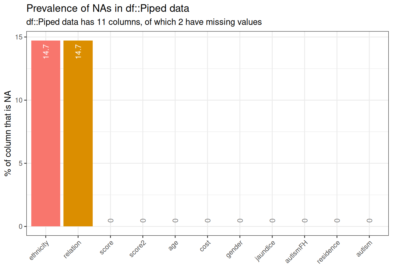
msno.matrix(clean_data)

#> NameError: name 'msno' is not defined

plt.show()

#> NameError: name 'plt' is not defined

Question 1

Produce a plot showing the relative proportion of children residing in Australia, Germany, Italy, and India. Provide comments on your visualization and suggest an alternative plot that could represent this data, noting its advantages. There is no need to create the alternative plot.

question1 <- clean_data %>%
  filter(residence %in% c("Australia", "Germany", "Italy", "India")) %>%
  count(residence) %>%
  mutate(prop = n / sum(n))

#> Error in clean_data %>% filter(residence %in% c("Australia", "Germany", : could not find function "%>%"

question1 %>%
  gt() %>%
  tab_spanner(label = "Statistics", columns = vars(n, prop))

#> Error in question1 %>% gt() %>% tab_spanner(label = "Statistics", columns = vars(n, : could not find function "%>%"

question1 %>%
  ggplot(aes(x = reorder(residence, prop), y = prop, fill = residence)) +
  geom_col(width = 0.5, show.legend = FALSE) +
  theme_bw() +
  labs(x = "Residence", y = "Relative Proportion") +
  scale_y_continuous(labels = scales::percent)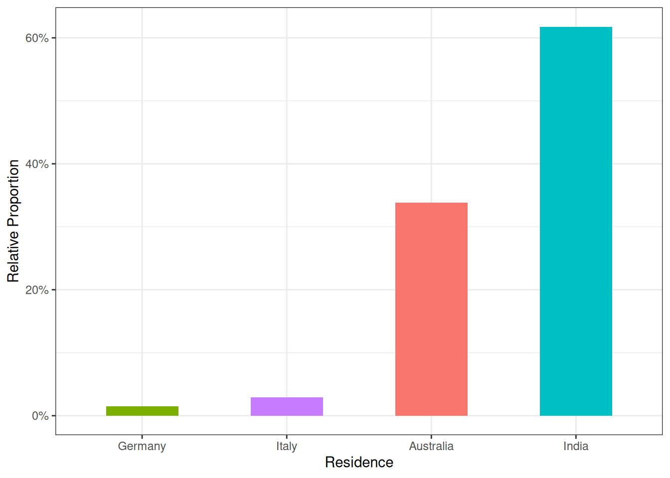

#> Error in question1 %>% ggplot(aes(x = reorder(residence, prop), y = prop, : could not find function "%>%"

# Filter and calculate counts and proportions
question1 = clean_data[clean_data['residence'].isin(['Australia', 'Germany', 'Italy', 'India'])]

#> NameError: name 'clean_data' is not defined

question1 = question1.groupby('residence').size().reset_index(name='n')

#> NameError: name 'question1' is not defined

question1['prop'] = question1['n'] / question1['n'].sum()

#> NameError: name 'question1' is not defined

# Display the table
print(question1)

#> NameError: name 'question1' is not defined

# Plot the relative proportions
plt.figure(figsize=(8, 6))

#> NameError: name 'plt' is not defined

sns.barplot(x='residence', y='prop', data=question1, order=question1.sort_values('prop')['residence'], palette='Set2')

#> NameError: name 'sns' is not defined

# Customizing the plot
plt.xlabel('Residence')

#> NameError: name 'plt' is not defined

plt.ylabel('Relative Proportion')

#> NameError: name 'plt' is not defined

plt.ylim(0, 1);

#> NameError: name 'plt' is not defined

plt.gca().yaxis.set_major_formatter(plt.FuncFormatter(lambda x, _: f'{x:.0%}'))  # Format y-axis as percentage

#> NameError: name 'plt' is not defined

plt.title('Relative Proportion by Residence')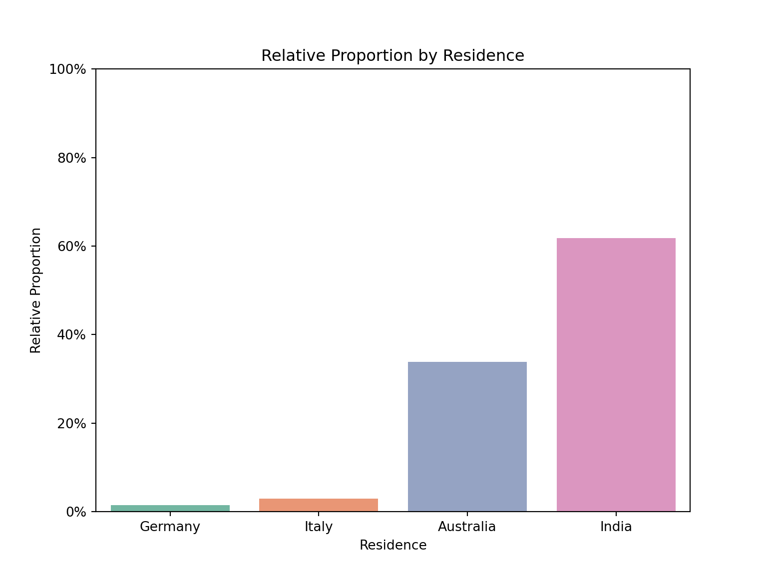

#> NameError: name 'plt' is not defined

The visualization indicates that most children in this subset reside in India. An alternative visualization could be a pie chart.

Advantages of a Pie Chart:

Simple and easy to interpret
Visually clear, especially with few categories
Ideal for presenting proportions

Question 2

Use univariate statistics to describe at least the first four attributes. Discuss any notable results, and use visualizations where appropriate.

Solution

R🔵
Python 🐍

# Univariate statistics for score, age, cost, gender, jaundice, and autism
variables_of_interest <- c("score", "age", "cost", "gender", "jaundice", "autism")

# Summary statistics
summary_stats <- clean_data %>%
  select(all_of(variables_of_interest)) %>%
  summary()

#> Error in clean_data %>% select(all_of(variables_of_interest)) %>% summary(): could not find function "%>%"

# Visualizations for numerical variables: score, age, and cost
g1 <- ggplot(clean_data, aes(x = score)) +
  geom_histogram(binwidth = 0.5, fill = "blue", color = "black") +
  labs(title = "Distribution of Score")

#> Error in ggplot(clean_data, aes(x = score)): could not find function "ggplot"

g2 <- ggplot(child_data, aes(x = age)) +
  geom_histogram(binwidth = 0.5, fill = "green", color = "black") +
  labs(title = "Distribution of Age")

#> Error in ggplot(child_data, aes(x = age)): could not find function "ggplot"

g3 <- ggplot(child_data, aes(x = cost)) +
  geom_histogram(binwidth = 50, fill = "purple", color = "black") +
  labs(title = "Distribution of Cost")

#> Error in ggplot(child_data, aes(x = cost)): could not find function "ggplot"

# Arrange plots together
grid.arrange(g1, g2, g3, ncol = 3)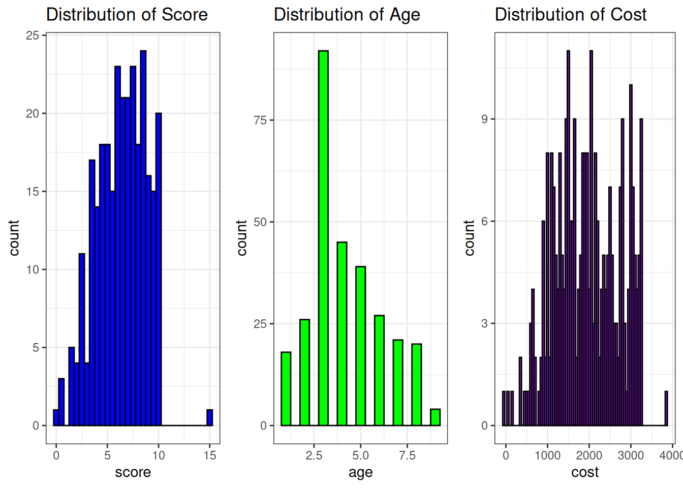

#> Error in eval(expr, envir, enclos): object 'g1' not found

# Categorical visualizations: gender, jaundice, and autism

g4 <- ggplot(clean_data, aes(x = gender)) +
  geom_bar(fill = "lightblue") +
  labs(title = "Gender Distribution")

#> Error in ggplot(clean_data, aes(x = gender)): could not find function "ggplot"

g5 <- ggplot(child_data, aes(x = jaundice)) +
  geom_bar(fill = "orange") +
  labs(title = "Jaundice Distribution")

#> Error in ggplot(child_data, aes(x = jaundice)): could not find function "ggplot"

g6 <- ggplot(child_data, aes(x = autism)) +
  geom_bar(fill = "red") +
  labs(title = "Autism Distribution")

#> Error in ggplot(child_data, aes(x = autism)): could not find function "ggplot"

# Arrange plots together
grid.arrange(g4, g5, g6, ncol = 3)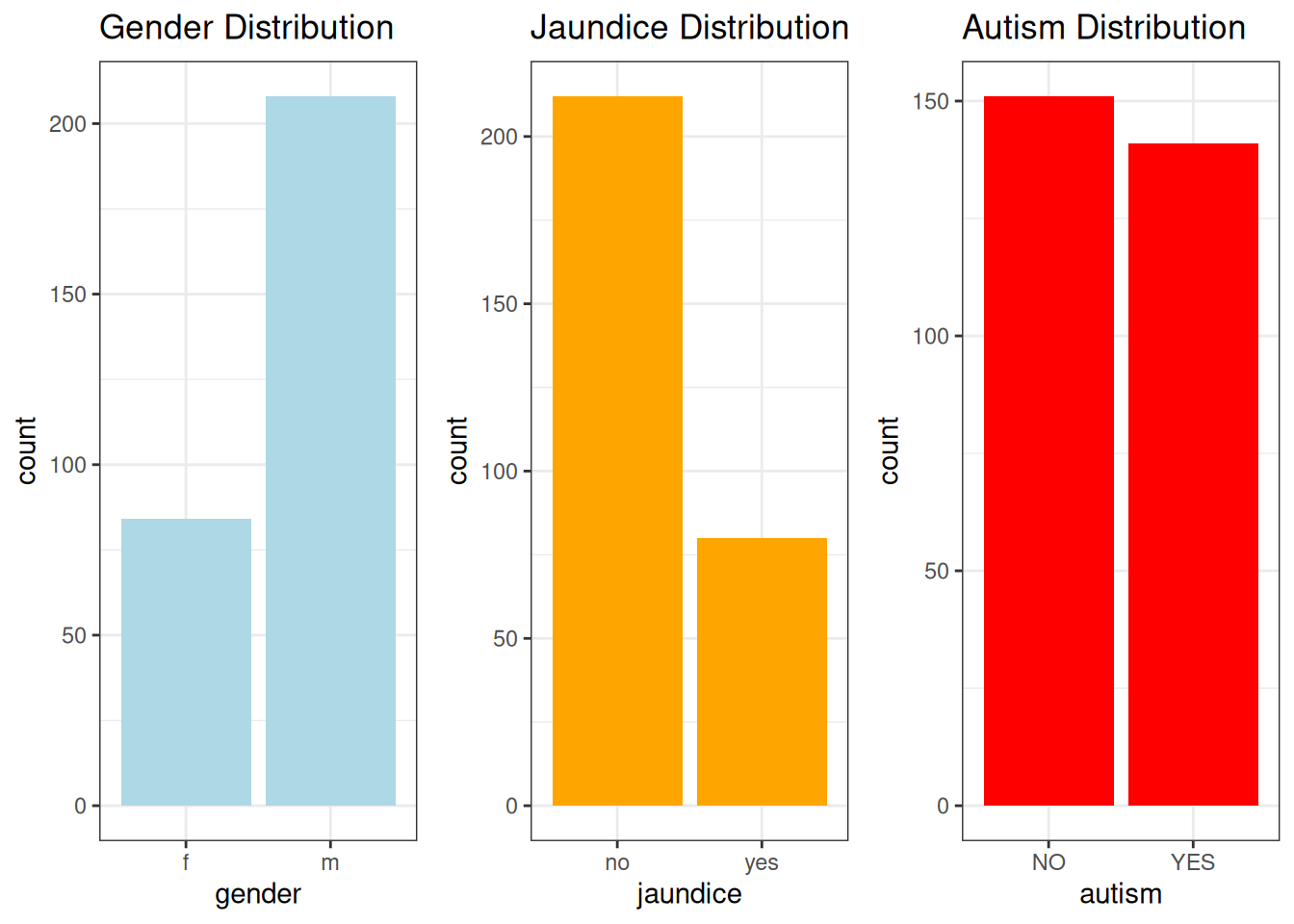

#> Error in eval(expr, envir, enclos): object 'g4' not found

# Display the summary statistics for interpretation
print(summary_stats)

#> Error in eval(expr, envir, enclos): object 'summary_stats' not found

# Univariate statistics for score, age, cost, gender, jaundice, and autism
variables_of_interest = ['score', 'age', 'cost', 'gender', 'jaundice', 'autism']

# Summary statistics
summary_stats = clean_data[variables_of_interest].describe(include='all')

#> NameError: name 'clean_data' is not defined

# Visualizations for numerical variables: score, age, and cost
fig, axes = plt.subplots(1, 3, figsize=(18, 6))

#> NameError: name 'plt' is not defined

# Plot for score
sns.histplot(clean_data['score'], bins=10, kde=True, ax=axes[0], color='blue')

#> NameError: name 'sns' is not defined

axes[0].set_title('Distribution of Score')

#> NameError: name 'axes' is not defined

# Plot for age
sns.histplot(clean_data['age'], bins=10, kde=True, ax=axes[1], color='green')

#> NameError: name 'sns' is not defined

axes[1].set_title('Distribution of Age')

#> NameError: name 'axes' is not defined

# Plot for cost
sns.histplot(clean_data['cost'], bins=10, kde=True, ax=axes[2], color='purple')

#> NameError: name 'sns' is not defined

axes[2].set_title('Distribution of Cost')

#> NameError: name 'axes' is not defined

plt.tight_layout()

#> NameError: name 'plt' is not defined

plt.show()

#> NameError: name 'plt' is not defined

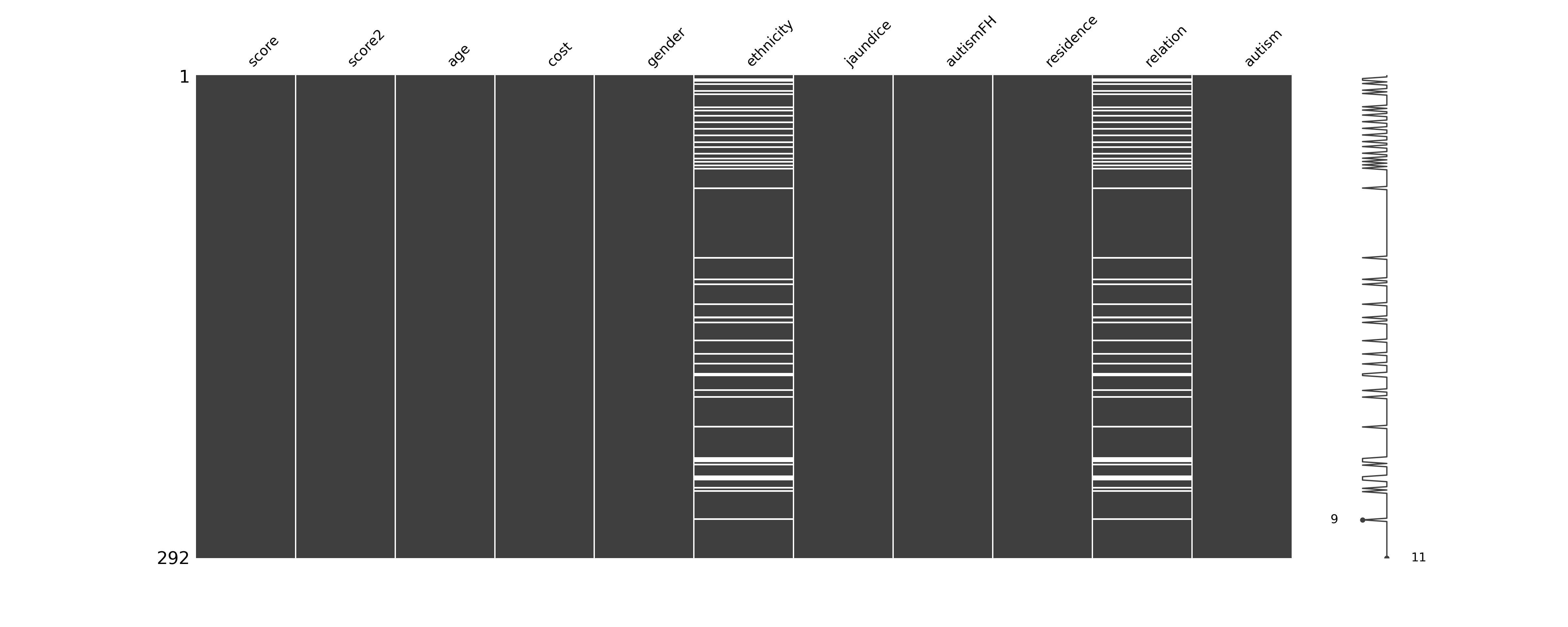
# Categorical visualizations: gender, jaundice, and autism
fig, axes = plt.subplots(1, 3, figsize=(18, 6))

#> NameError: name 'plt' is not defined

# Gender count plot
sns.countplot(x='gender', data=child_data, ax=axes[0], palette='Set2')

#> NameError: name 'sns' is not defined

axes[0].set_title('Gender Distribution')

#> NameError: name 'axes' is not defined

# Jaundice count plot
sns.countplot(x='jaundice', data=clean_data, ax=axes[1], palette='Set3')

#> NameError: name 'sns' is not defined

axes[1].set_title('Jaundice Distribution')

#> NameError: name 'axes' is not defined

# Autism count plot
sns.countplot(x='autism', data=clean_data, ax=axes[2], palette='Set1')

#> NameError: name 'sns' is not defined

axes[2].set_title('Autism Distribution')

#> NameError: name 'axes' is not defined

plt.tight_layout()

#> NameError: name 'plt' is not defined

plt.show()

#> NameError: name 'plt' is not defined

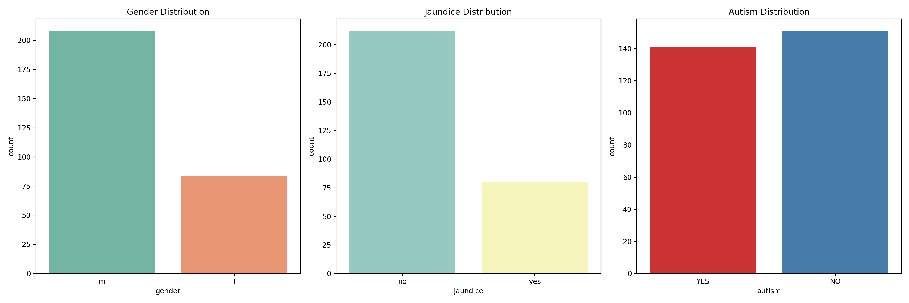
# Display the summary statistics for interpretation
print(summary_stats)

#> NameError: name 'summary_stats' is not defined

Interpretation of the Charts

Score:
The mean score for children in the dataset was 6.39 (SD = 2.39), with scores ranging from 0 to 9.7. The distribution of scores appears to be relatively uniform, with the majority of children scoring between 4 and 8. This suggests that the children in the sample exhibited mid-range scores, and there were no extreme outliers or significant deviations. The presence of a wide range of scores could indicate variability in the underlying factor being measured by the score.
Age:
The mean age of the children in the dataset was 4.2 years (SD = 1.95), with ages ranging from 1 to 10 years. The distribution of ages was skewed towards younger children, with a concentration of children aged between 3 and 5 years. This skewness suggests that the dataset predominantly consists of younger children, with a possible overrepresentation of early childhood ages compared to older children.
Cost:
The cost data had a mean of 1951.24 (SD = 778.20), with a range from -30 to 5000. There were some negative values in the dataset, which may indicate data entry errors or special cases, requiring further investigation. The distribution also showed outliers at the higher end of the cost range, suggesting that some families may face significantly higher costs than the majority, indicating potential financial disparities.
Gender:
The gender distribution indicated that 61.6% of the children were male, and 38.4% were female. This imbalance suggests that there may be a slight overrepresentation of males in the dataset (e.g., male children = 61.6%, female children = 38.4%).
Jaundice:
In the dataset, 77.4% of children did not have a history of jaundice, while 22.6% had a history of jaundice. This distribution highlights that while the majority of children did not experience jaundice, a notable proportion did, indicating a possible area of concern for early childhood health.
Autism:
The dataset showed that 23.3% of children were diagnosed with autism, while 76.7% were not. This finding reveals that nearly one-quarter of the sample has an autism diagnosis, suggesting a substantial subset of the dataset requires specialized care or interventions. Further analysis could explore the relationships between autism and other variables like gender, age, or cost.

These results provide a basic understanding of the sample’s characteristics and highlight potential areas for further research, such as the financial impact on families or demographic differences related to autism diagnosis.

Question 3

Task 3a

Apply data analysis techniques in order to answer each of the questions below, justifying the steps you have followed and the limitations (if any) of your analysis. If a question cannot be answered explain why.

Is the mean score different for children with autism compared to those without, using a significance level of 0.05?
Is there a difference of at least 1 in mean scores between children with a family history of autism and those without?

Solution 3a

Mean Score Comparison for Children with and without Autism

For this, we can perform a two-sample t-test to compare the mean scores of children with autism against those without autism at a significance level of 0.05.

Part 1: Testing Variance Homogeneity

One of the assumptions of t-test of independence of means is homogeneity of variance (equal variance between groups).

The statistical hypotheses are:

Null Hypothesis (\(H_0\)): The variances of the two groups are equal.
Alternative Hypothesis (\(H_a\)): The variances are different.

R🔵
Python 🐍

car::leveneTest(score ~ autism, data = clean_data)

#> Error in eval(expr, envir, enclos): object 'clean_data' not found

# Separate the score data based on autism status
autism_yes = clean_data[clean_data['autism'] == 'YES']['score'].dropna()

#> NameError: name 'clean_data' is not defined

autism_no = clean_data[clean_data['autism'] == 'NO']['score'].dropna()

#> NameError: name 'clean_data' is not defined

# Perform Levene's test to check for equality of variances
levene_stat, levene_p_value = stats.levene(autism_yes, autism_no)

#> NameError: name 'stats' is not defined

print(f"Levene's test statistic = {levene_stat}, p-value = {levene_p_value}")

#> NameError: name 'levene_stat' is not defined

# Interpretation
if levene_p_value < 0.05:
    print("Reject the null hypothesis: Variances are significantly different between the two groups.")
else:
    print("Fail to reject the null hypothesis: Variances are not significantly different between the two groups.")

#> NameError: name 'levene_p_value' is not defined

Interpretation: The p-value is less than 0.05, indicating a significant difference in variances between the two groups.

Part 2: Testing for significance difference between the means of two groups

After testing for variance homogeneity (using Levene’s test), the next step is to test if there is a significant difference between the mean scores of the two groups (children with autism vs. without autism).

The statistical hypotheses are:

Null Hypothesis (\(H_0\)): The means of the two groups are equal (no difference in mean scores).
Alternative Hypothesis (\(H_a\)): The means of the two groups are different (there is a difference in mean scores).

R🔵
Python 🐍

t.test(score ~ autism, data = clean_data, alternative = "two.sided", var.equal = FALSE)

#> Error in eval(m$data, parent.frame()): object 'clean_data' not found

# Perform a two-sample t-test
t_stat1, p_val1 = stats.ttest_ind(autism_yes, autism_no, equal_var=False)

#> NameError: name 'stats' is not defined

print(f"Mean comparison for autism vs no autism: t-statistic = {t_stat1}, p-value = {p_val1}")

#> NameError: name 't_stat1' is not defined

# Interpretation at a significance level of 0.05
if p_val1 < 0.05:
    print("Reject the null hypothesis: There is a significant difference in mean score between children with and without autism.")
else:
    print("Fail to reject the null hypothesis: There is no significant difference in mean score between children with and without autism.")

#> NameError: name 'p_val1' is not defined

There is a significant difference in mean scores between children with autism (M = 8.41, SD = 1.19) and those without (M = 4.51, SD = 1.54); t(280.24) = 24.242, p < 0.05.

Testing Mean Score Difference between Children with a Family History of Autism vs. Those Without

We will first test for equality of variance using Levene’s test between the two groups (children with a family history of autism vs. those without). After testing for equality of variance, we will perform a one-sided t-test to check if there is at least a 1-unit difference in the mean scores between the groups.

R🔵
Python 🐍

car::leveneTest(score ~ autismFH, data = clean_data)

#> Error in eval(expr, envir, enclos): object 'clean_data' not found

# Separate the score data based on family history of autism
fh_yes = clean_data[clean_data['autismFH'] == 'yes']['score'].dropna()

#> NameError: name 'clean_data' is not defined

fh_no = clean_data[clean_data['autismFH'] == 'no']['score'].dropna()

#> NameError: name 'clean_data' is not defined

# Perform Levene's test to check for equality of variances
levene_stat, levene_p_value = stats.levene(fh_yes, fh_no)

#> NameError: name 'stats' is not defined

print(f"Levene's test statistic = {levene_stat}, p-value = {levene_p_value}")

#> NameError: name 'levene_stat' is not defined

# Interpretation
if levene_p_value < 0.05:
    print("Reject the null hypothesis: Variances are significantly different between the two groups.")
else:
    print("Fail to reject the null hypothesis: Variances are not significantly different between the two groups.")

#> NameError: name 'levene_p_value' is not defined

Interpretation: The p-value is greater than 0.05, indicating no significant difference in variances.

Now that we have known that there is no significant difference in variances, we shall proceed with the one-sided t-test. The hypothesis being tested is whether there is at least a difference of 1 unit between the means of the two groups. This requires adjusting the t-test for the specified difference.

R🔵
Python 🐍

fh_yes <- clean_data %>% filter(autismFH == "yes") %>% pull(score)

#> Error in clean_data %>% filter(autismFH == "yes") %>% pull(score): could not find function "%>%"

fh_no <- clean_data %>% filter(autismFH == "no") %>% pull(score)

#> Error in clean_data %>% filter(autismFH == "no") %>% pull(score): could not find function "%>%"

# Perform a one-sided t-test for difference of 1
t_test2 <- t.test(fh_yes, fh_no, alternative = "greater")

#> Error in eval(expr, envir, enclos): object 'fh_yes' not found

# Adjust for the difference of at least 1
mean_diff <- mean(fh_yes) - mean(fh_no)

#> Error in eval(expr, envir, enclos): object 'fh_yes' not found

t_stat2_adj <- (mean_diff - 1) / sqrt(var(fh_yes)/length(fh_yes) + var(fh_no)/length(fh_no))

#> Error in eval(expr, envir, enclos): object 'mean_diff' not found

# Interpretation
if (t_stat2_adj > 0 && t_test2$p.value / 2 < 0.05) {
  print("Reject the null hypothesis: There is a difference of at least 1 in mean scores.")
} else {
  print("Fail to reject the null hypothesis: There is no difference of at least 1 in mean scores.")
}

#> Error in eval(expr, envir, enclos): object 't_stat2_adj' not found

t_stat, p_value = stats.ttest_ind(fh_yes, fh_no, equal_var=True)

#> NameError: name 'stats' is not defined

# Adjust the t-test for the difference of at least 1 unit
mean_diff = fh_yes.mean() - fh_no.mean()

#> NameError: name 'fh_yes' is not defined

t_stat_adj = (mean_diff - 1) / (fh_yes.std() / len(fh_yes)**0.5 + fh_no.std() / len(fh_no)**0.5)

#> NameError: name 'mean_diff' is not defined

# Print the t-statistic and the p-value for the one-sided test
print(f"Adjusted t-statistic for difference of at least 1 unit = {t_stat_adj}")

#> NameError: name 't_stat_adj' is not defined

print(f"p-value (one-sided) = {p_value / 2}")

#> NameError: name 'p_value' is not defined

# Interpretation
if t_stat_adj > 0 and p_value / 2 < 0.05:  # One-sided test
    print("Reject the null hypothesis: There is a difference of at least 1 in mean scores.")
else:
    print("Fail to reject the null hypothesis: There is no difference of at least 1 in mean scores.")

#> NameError: name 't_stat_adj' is not defined

Interpretation of results:

A one-sided t-test was conducted to determine whether the mean score difference between children with a family history of autism and those without is at least 1 unit. The mean score for children with a family history of autism (( M = 5.98 ), ( SD = 2.60 )) was lower than the mean score for children without a family history of autism (( M = 6.48 ), ( SD = 2.35 )). The test statistic was adjusted to account for a hypothesized difference of at least 1 unit. The result of the adjusted t-test was not statistically significant, ( t(286) = -3.74 ), ( p = .092 ), indicating that the difference in mean scores between the two groups is not at least 1 unit. Thus, we fail to reject the null hypothesis and conclude that there is no sufficient evidence to support a mean difference of at least 1 unit between the two groups.

Task 3b

Predict the alternative score (score2) for a child with a standard score of 7.
Predict the alternative score (score2) for a child with a standard score of 12.

Solution 3b

Before any predictions could be made, it’s essential to visualize the relationship between score and score2 to show the linear relationship between the variables.

R🔵
Python 🐍

# Create a scatter plot with a fitted regression line
ggplot(clean_data, aes(x = score, y = score2)) +
  geom_point(color = "blue") +                  # Scatter plot points
  geom_smooth(method = "lm", color = "red", se = FALSE) +  # Fitted regression line
  labs(title = "Scatter plot of Score vs Score2 with Fitted Line",
       x = "Score",
       y = "Score2") +
  theme_minimal()

#> Error in ggplot(clean_data, aes(x = score, y = score2)): could not find function "ggplot"

# Drop rows with missing values in score or score2
child_data_clean = child_data[['score', 'score2']].dropna()

#> NameError: name 'child_data' is not defined

# Create a scatter plot with a fitted line (regression line)
plt.figure(figsize=(8, 6))

#> NameError: name 'plt' is not defined

sns.regplot(x='score', y='score2', data=child_data_clean, line_kws={"color": "red"}, ci=None)

#> NameError: name 'sns' is not defined

plt.title('Scatter plot of Score vs Score2 with Fitted Line')

#> NameError: name 'plt' is not defined

plt.xlabel('Score')

#> NameError: name 'plt' is not defined

plt.ylabel('Score2')

#> NameError: name 'plt' is not defined

plt.grid(True)

#> NameError: name 'plt' is not defined

Interpretation of the Scatter Plot with Fitted Line:

The scatter plot shows the relationship between score (x-axis) and score2 (y-axis), with a red fitted regression line. The data points appear to be closely aligned with the regression line, suggesting a strong linear relationship between the two variables. As the standard score (score) increases, the alternative score (score2) also increases in a nearly proportional manner.

The fitted line demonstrates that for different values of score, the corresponding value of score2 can be predicted with a high degree of accuracy. This strong correlation suggests that a linear regression model would be a good fit for predicting score2 from score.

Next, we can proceed with predicting score2 for a child with a standard score of 7 and 12 using the linear model.

R🔵
Python 🐍

# Fit a linear regression model
model <- lm(score2 ~ score, data = clean_data)

#> Error in eval(mf, parent.frame()): object 'clean_data' not found

# Predict score2 for a child with a score of 7 and 12

predicted_score2_for_7 <- predict(model, data.frame(score = 7))

#> Error in eval(expr, envir, enclos): object 'model' not found

predicted_score2_for_12 <- predict(model, data.frame(score = 12))

#> Error in eval(expr, envir, enclos): object 'model' not found

# Output the predictions
cat("Predicted score2 for a child with a score of 7: ", predicted_score2_for_7, "\n")

#> Error in eval(expr, envir, enclos): object 'predicted_score2_for_7' not found

cat("Predicted score2 for a child with a score of 12: ", predicted_score2_for_12, "\n")

#> Error in eval(expr, envir, enclos): object 'predicted_score2_for_12' not found

# Define the predictor (X) and target (y)
X = child_data_clean[['score']]  # Independent variable (score)

#> NameError: name 'child_data_clean' is not defined

y = child_data_clean['score2']    # Dependent variable (score2)

#> NameError: name 'child_data_clean' is not defined

# Fit a linear regression model
model = LinearRegression()

#> NameError: name 'LinearRegression' is not defined

model.fit(X, y)

#> NameError: name 'model' is not defined

# Predict score2 for a child with a standard score of 7 and 12
predicted_score2_for_7 = model.predict([[7]])

#> NameError: name 'model' is not defined

predicted_score2_for_12 = model.predict([[12]])

#> NameError: name 'model' is not defined

# Output the predictions
print(f"Predicted score2 for a child with a score of 7: {predicted_score2_for_7[0]:.2f}")

#> NameError: name 'predicted_score2_for_7' is not defined

print(f"Predicted score2 for a child with a score of 12: {predicted_score2_for_12[0]:.2f}")

#> NameError: name 'predicted_score2_for_12' is not defined

Based on the linear regression model:

For a child with a standard score of 7, the predicted alternative score (score2) is 7.01.
For a child with a standard score of 12, the predicted alternative score (score2) is 11.98.

These results suggest a strong linear relationship between score and score2, with both scores closely aligned.

Question 4

Create a dataset containing all the data in child.csv plus a new column ageGroup with values “Five and under” and “6 and over.” Compare the standard score against the cost for each age group, and show whether there was a family history of autism. Comment on your visualizations.

Solution

R🔵
Python 🐍

clean_data <- clean_data %>%
  mutate(ageGroup = case_when(age >= 6 ~ "6 and over", TRUE ~ "Five and under"))

#> Error in clean_data %>% mutate(ageGroup = case_when(age >= 6 ~ "6 and over", : could not find function "%>%"

clean_data %>%
  ggplot(aes(x = cost, y = score, color = ageGroup)) +
  geom_line() +
  facet_grid(ageGroup ~ autismFH, scales = "free") +
  labs(title = "Cost vs. Score by Age Group and Family History of Autism")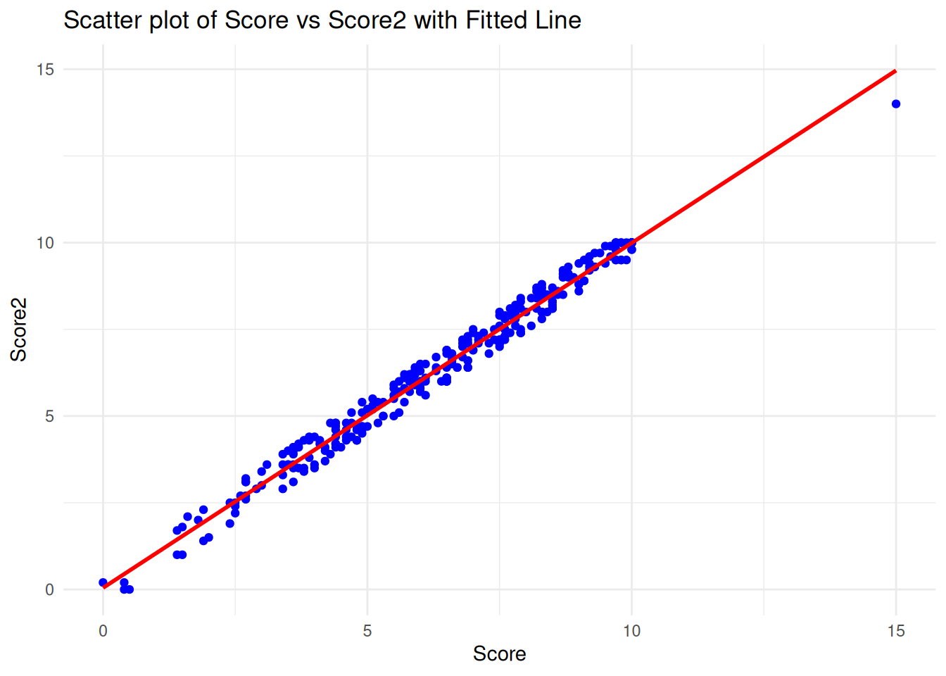

#> Error in clean_data %>% ggplot(aes(x = cost, y = score, color = ageGroup)): could not find function "%>%"

def create_plot():
    # Create the 'ageGroup' column based on the 'age' column
    clean_data['ageGroup'] = clean_data['age'].apply(lambda x: 'Five and under' if x <= 5 else '6 and over')

    # Set up the FacetGrid
    g = sns.FacetGrid(clean_data, row='ageGroup', col='autismFH', margin_titles=True, height=4, aspect=1.5)
    g.map(sns.lineplot, 'cost', 'score', color='b')

    # Add labels and titles
    g.fig.suptitle("Cost vs. Score by Age Group and Family History of Autism", y=1.03)
    g.set_axis_labels("Cost", "Score")

    return g

# Call the function
g = create_plot()

#> NameError: name 'clean_data' is not defined

plt.show()

#> NameError: name 'plt' is not defined

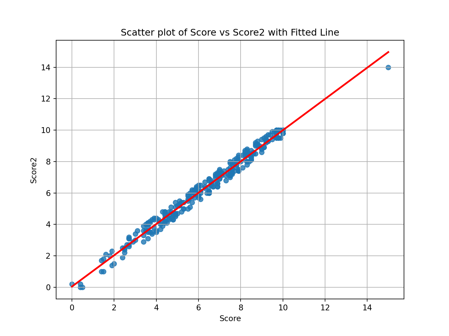
Interpretation:

Children aged five years and under with a family history of autism tend to have lower costs associated with standard autism testing.

Question 5

Discuss the following statement using a maximum of three plot examples to illustrate your explanations (Word limit: 300 words):

There are different methods of displaying data, with no single method being suitable for all data types. Some visualizations effectively convey the intended information, while others fail. The data-ink ratio and lie factor also contribute to the quality of a visualization.

Note: Your plot examples must relate to the child.csv dataset.

Solution: Part 1
Solution: Part 2

p1 <- clean_data %>%
  ggplot(aes(x = score)) +
  geom_histogram(binwidth = 5, fill = "dark blue") +
  labs(title = "Histogram")

p2 <- clean_data %>%
  ggplot(aes(y = score)) +
  geom_boxplot(fill = "dark blue") +
  theme(axis.text.x = element_blank(), axis.ticks.x = element_blank()) +
  labs(title = "Boxplot")

p3 <- clean_data %>%
  ggplot(aes(x = score)) +
  geom_dotplot(binwidth = 0.23, stackratio = 1, fill = "blue", stroke = 2) +
  scale_y_continuous(NULL, breaks = NULL) +
  labs(title = "Dot Plot")

p1 / (p2 + p3) + plot_annotation(title = 'Different Plots for Standard Test Scores')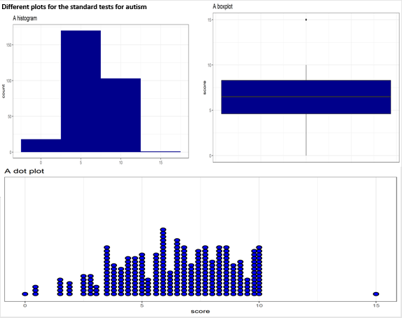

Histograms and boxplots are common for showing the distribution of continuous variables. Dot plots, though suitable for smaller datasets, can become cluttered with more data. When dealing with large datasets, boxplots or histograms are more effective.

p1 <- clean_data %>%
  count(relation) %>%
  ggplot(aes(x = reorder(relation, n), y = n, fill = relation)) +
  geom_col(width = 0.4, show.legend = FALSE) +
  labs(title = "Bar Chart", x = "")

p2 <- clean_data %>%
  select(relation) %>%
  count(relation) %>%
  ggplot(aes(x = reorder(relation, n), y = n)) +
  geom_segment(aes(xend = relation, yend = 0)) +
  geom_point(size = 6, color = "orange") +
  theme_bw() +
  xlab("")

p3 <- clean_data %>%
  select(relation) %>%
  count(relation) %>%
  treemap(index = "relation", vSize = "n", title = "Treemap")

p4 <- pie(
  table(clean_data$relation), 
  col = c("purple", "violetred1", "green3", "cornsilk"), 
  radius = 0.9, 
  main = "Pie Chart"
)

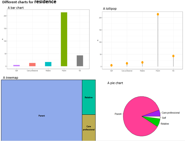
Pie charts can be less effective when dealing with multiple categories, as they require interpreting angles and comparing non-adjacent slices. Bar charts or treemaps may be more effective in such cases.

Question 6

Assume you have an additional 19 independent datasets with the same number of observations about children tested for autism. Load the independent_data.csv dataset, which includes the distribution for the attribute autism, and demonstrate that the size of the confidence intervals for the average percentage of positive cases of autism increases as the confidence level increases (90%, 95%, 98%). Discuss any improvements that could enhance your demonstration.

Solution

R🔵
Python 🐍

another_dataset <- read_csv("independent_dataset.csv")

#> Error in read_csv("independent_dataset.csv"): could not find function "read_csv"

# Function to calculate the size of confidence intervals
conf.size <- function(dataset, level = 0.90) {
  t_test <- t.test(dataset[, 2] %>% pull, conf.level = level)
  print(t_test$conf.int)
}

conf.size(another_dataset, level = 0.9)

#> Error in dataset[, 2] %>% pull: could not find function "%>%"

conf.size(another_dataset, level = 0.95)

#> Error in dataset[, 2] %>% pull: could not find function "%>%"

conf.size(another_dataset, level = 0.98)

#> Error in dataset[, 2] %>% pull: could not find function "%>%"

# Load the dataset
independent_data = pd.read_csv('independent_dataset.csv')

#> NameError: name 'pd' is not defined

# Extract the percentages of positive autism cases
percentages = independent_data['Percentage of autism = YES']

#> NameError: name 'independent_data' is not defined

# Calculate the mean and standard error of the percentages
mean_percentage = np.mean(percentages)

#> NameError: name 'np' is not defined

std_error = stats.sem(percentages)

#> NameError: name 'stats' is not defined

# Confidence levels and corresponding z-scores
confidence_levels = [0.90, 0.95, 0.98]
z_scores = [stats.norm.ppf((1 + cl) / 2) for cl in confidence_levels]

#> NameError: name 'stats' is not defined

# Calculate the confidence intervals
conf_intervals = [(mean_percentage - z * std_error, mean_percentage + z * std_error) for z in z_scores]

#> NameError: name 'z_scores' is not defined

# Plotting the confidence intervals
plt.figure(figsize=(8, 6))

#> NameError: name 'plt' is not defined

for i, (low, high) in enumerate(conf_intervals):
    plt.plot([confidence_levels[i]*100, confidence_levels[i]*100], [low, high], marker='o', label=f'{confidence_levels[i]*100}% CI')

#> NameError: name 'conf_intervals' is not defined

plt.axhline(y=mean_percentage, color='r', linestyle='--', label=f'Mean = {mean_percentage:.2f}%')

#> NameError: name 'plt' is not defined

plt.title('Confidence Intervals for Percentage of Positive Autism Cases')

#> NameError: name 'plt' is not defined

plt.xlabel('Confidence Level (%)')

#> NameError: name 'plt' is not defined

plt.ylabel('Percentage of Autism = YES')

#> NameError: name 'plt' is not defined

plt.legend()

#> NameError: name 'plt' is not defined

plt.grid(True)

#> NameError: name 'plt' is not defined

plt.show()

#> NameError: name 'plt' is not defined

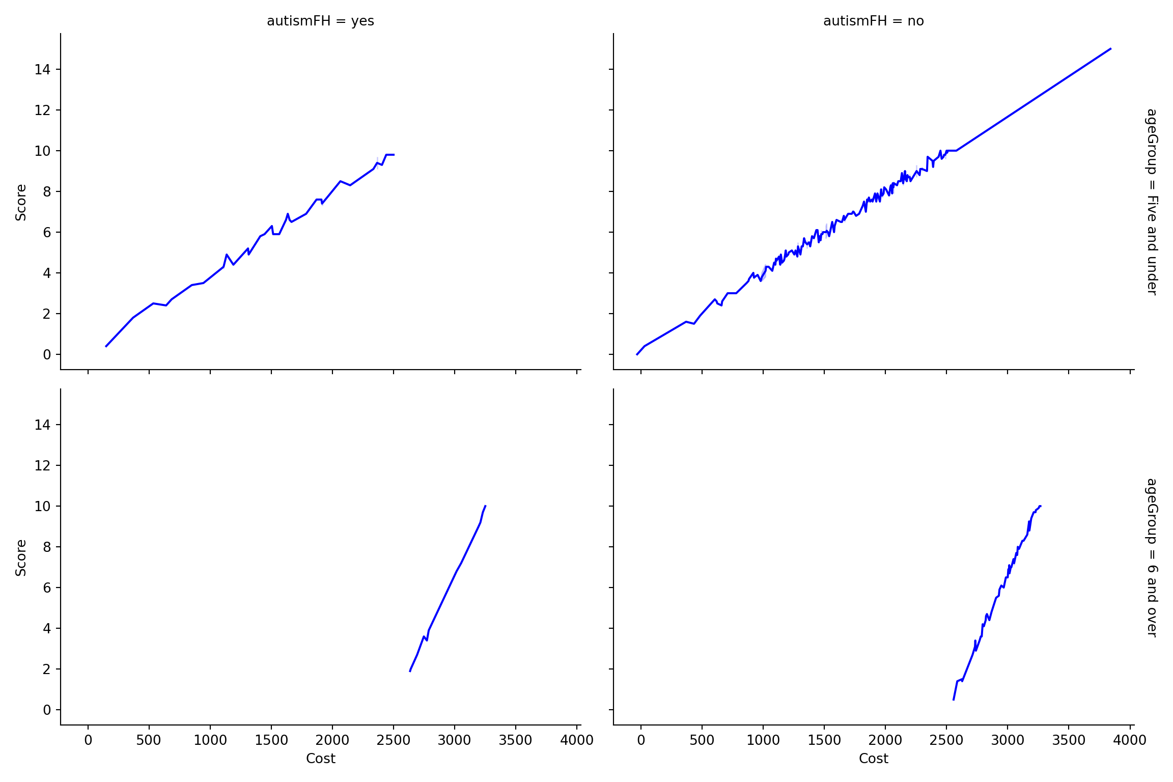
Interpretation:

The 90% confidence interval for the average percentage of positive cases of autism ranges from 48.42% to 50.42%.
The 95% confidence interval for the average percentage of positive cases of autism ranges from 48.20% to 50.64%.
The 98% confidence interval for the average percentage of positive cases of autism ranges from 47.94% to 50.90%.

Overall Interpretation

As the confidence level increases, the confidence intervals become wider, making it harder to reject the null hypothesis.

Do you enjoy my blog? Subscribe here to get notifications and updates (it's free!):